Winning Basketball
Predicting NBA game outcomes using machine learning

The objective of every coach is to win. Pre-game and in-game, they must decide which players deserve more minutes so the team can improve in key performance areas, and by extension, which areas should be focused on.
My goal was to predict ‘win’ or ‘loss’, taking measures of performance as input. The final model correctly classified 84.44% of unseen game data.
Coaches can estimate team performance categories, use this model to predict the outcome, then shuffle their lineups to target certain categories in their control that will output winning predictions.
My assumptions are that coaches can aggregate each player’s season averages to accurately estimate:
- The performance of the opposing lineup
- The performance of their own lineup
Dataset
The dataset (games.csv) contains information on 23,195 NBA games from every season between 2003–2019.
This was randomly split into a train set (80% of data) to learn from, and a test set (20% of data) to evaluate performance. Further, this was split into X_train/X_test (features), and y_train/y_test (target).
Features
For each game (row), we have the following features (columns) for both home and away teams:
FG_PCT_home/FG_PCT_away: % of made shots (excluding free throws)FT_PCT_home/FT_PCT_away: % of made free throwsFG3_PCT_home/FG3_PCT_away: % of made 3-point shotsAST_home/AST_away: # of assistsREB_home/REB_away: # of rebounds
I wanted to predict the HOME_TEAM_WINS column (target); assuming that ours is always the home team. A 0 represents a loss, and a 1 represents a win.
Dropped Games
The train set was missing data for 77 games. Estimating each feature of these games would detract from the analysis, so they were dropped. I also dropped one game with an erroneous 36–33 score.
Outliers
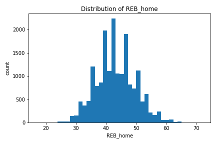
The following histograms display, for each feature, the count of values in a bin (value range). Most are centered, meaning there are no values far outside the middle that shift the distribution (potential outliers).


There are some games with very low FT_PCT, shifting the distribution right. These are real; NBA games typically have high FT_PCT with occasional bad performances. They were kept because eliminating them would artificially divorce our data from reality.


Some games had high FG3_PCT or REB, shifting the following distributions left, but they too were kept. Teams usually shoot a low FG3_PCT, but with few 3-point attempts, an accuracy of 1.0 is possible. Likewise, overtime games allow teams to collect supernormal rebounds.


Outcome Splits by Feature
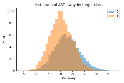
I then separated histograms by outcome, where orange represents values recorded in wins; and blue in losses.


FG_PCT_home shows that games with high efficiency are overwhelmingly won (orange). FG_PCT_away is the reverse; games where the opponents had high efficiency are overwhelmingly lost (blue). Similar splits appear for the following features, but the relationship is less strong.


Model
Preprocessing
Input transformations improve the model’s ability to learn.
The preproc_pipe takes inputs, fills in missing values with the median of that feature from the train set, and then squishes every value into a distribution that has a mean of 0 and a standard deviation of 1 (standard normal distribution). This second step (scaling) prevents the model from artificially favoring features like REB_home/REB_away that are larger.
Model Selection
After trying multiple approaches (LGBMClassifier, LogisticRegression, RandomForestClassifier) and settings (hyperparameters) for each, the best model was LogisticRegression with default settings.
LogisticRegression defines a linear equation where the outputs (y) lie between 0 and 1. Outputs ≥ 0.5, are classified as wins (1) and outputs < 0.5 as losses (0). When training, coefficients are continuously tweaked to minimize the difference between actual and predicted values. Then, it can multiply unseen inputs by trained parameters, and predict.
The final line splits train into 10 chunks. For each of 10 iterations, the model preprocesses the inputs, then trains LogisticRegression on 9/10 chunks before validating performance on the 10th (unseen) chunk. Using different validation chunks each iteration allows for more training on limited data, and increased confidence in results.
Results
Train Set
This model should beat the baseline accuracy (% correct predictions) of 59% (obtained by always predicting the most frequent outcome, wins).
Above, we see average scores on the validation chunk are close to average scores on the training chunks. This means our model has not overfit; it performs similarly on unseen data. In the train set:
- It correctly classified 83.83% of games (
validation_accuracy) - Of ‘win’ classifications, 85.61% were truly won (
validation_precision) - It identified 87.52% of actual wins (
validation_recall)
The average difference in accuracy across validation chunks (standard deviation) was small: 0.007263.
Test Set
On the 20% of data the model had never seen, it correctly classified 84.44% of game outcomes, which was close (within standard deviation) to the train set (83.83%). This again builds confidence that our model has not overfit.
Feature Importances
The below visualization shows the impact of each feature (its coefficient) on prediction; something that might interest coaches.

Larger positive coefficients influence the model to predict wins, whereas negative coefficients influence the model to predict losses. As before, FG_PCT had the highest impact on predictions; greater FG_PCT_home influences the model to predict ‘win’, and greater FG_PCT_away influences the model to predict ‘loss’. AST_home/AST_away were the least important features because they had the smallest magnitude of impact.
Caveats
Assumptions
Given the starting assumptions, accurate models might not help decision-making if coaches poorly estimate the performances of lineups.
Features
Other features could significantly impact outcomes; especially defensive statistics like steals and blocks. A richer dataset could mitigate this weakness.
Fundamental Changes
New rules and strategies constantly redefine the NBA, like the recent popularity of the 3-point shot. Changes in gameplay trends can reduce future predictive power, as the data becomes fundamentally different.
Full code available here.
